Parameter Optimization in Catchment-CN4.5

Figure 1. Global Plant Functional Types

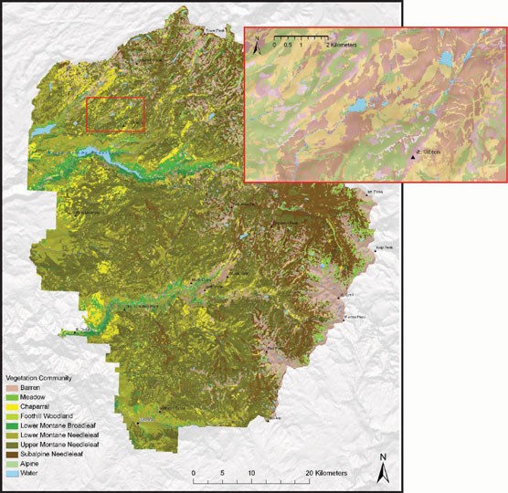
Figure 2. Yosemite National Park Vegetation Map
The Catchment project is research into improving land surface model parameters that represent vegetation processes. In particular this project looked at finding a globally applicable linear combination of existing local environmental factors tp predict vegetation parameters. The linear coefficients were computed to provide an optimal estimate of the stomatal marginal water use efficiency, g1, across the continental United States. It is optimal in the sense that the the linear coefficients that predict g1 were optimized to minimize the sum of the relative mean average error for streamflow over each basin and the relative mean average error of evapotranspiration over all Catchment-CN4.5 pixels. Alternative approaches to this model generally use just a single parameter for each single plant functional type, as illustrated in the map above in Figure 1. from De Kauwe et al, which displays one way that plant functional types are assigned to regions in the continental United States. But as an example of the range of local diversity of plants, Figure 2. above provides a vegetation map of Yosemite National park, which is the result of reducing 129 unique vegetation classes into 8 broad vegetation types. This research was motivated by using local climate measures to incorporate local diversity.
The linear model for g1 has a scale factor for each of the 7 plant functional types (PFT), denoted as ai for i=1, 2, …, 7. The scaling factor is used to avoid compensating errors in the overall model. Researchers’ early modeling efforts demonstrated that the optimization algorithm worked best when the number of ai and bk parameters were kept to as few as possible. Therefore, they chose to use only 2 environmental factors: mean annual precipitation and canopy height. Previous analyses showed that these were both important predictors of g1 globally. The resulting modeling equations for g1 then had the following form:
g1 (s) = ai * (b0 + b1 * precip(s) + b2 * CanopyHeight(s) ),
where s is the catchment-CN4.5 pixel and i is the PFT.
That is, there are 7 scaling factors and three linear coefficients to be determined. One can think of this as finding a point in a 10-dimensional space 0r a 10-tuple, (a1, a2, a3, a4, a5, a6, a7, b0, b1, b2) that will minimize the relative mean average error described. As described below, we will refer to this 10-tuple as a “particle”, so as to be consistent wit the optimization method used. and avoid confusion with the reference of a point within Catchment-CN4.5.
This type of optimization problem requires heuristic based methods. These usually require concurrently running a model at many different settings of the parameters that are trying to be determined (in this case the scaling factors and linear coefficients) and using a heuristic-based method to identify a new set of points and to continue iterating until there is no further improvement in the solution, which is what also defines convergence for the method. In this research the Particle Swarm Optimization (PSO) method was used. The different settings or scaling factors and linear coefficients are referred to as swarm particles in the POS method. Researchers began their analysis using 10 swarm particles. Over time it was identified that 30 swarm particles were required to achieve convergence beyond local minimums.
Each individual run for a swarm particle, ran for eight hours on an 8-core node with 64GiB of memory, with a 4.245 Gibps storage bandwidth. These individual runs shared 1.2 TB of AWS’s FSx Lustre. Over 14,500 total compute node hours were required. It was estimated that running this optimization process on premises without making significant changes to the code would result in individual iterations requiring up to a week to complete because of wait times for the 30 distributed jobs, meaning that convergence might require over 10 weeks of flow time to finish. With the expectation that there would be several convergence efforts, on premises computing was considered infeasible. In the cloud, without making any code changes, each iteration would complete in 8 hours using a total of 240 compute node hours. In this research effort there were at least 60 iterations performed overall.
Required data was uploaded to AWS in April of 2023. There were significant issues in using Spack to build the infrastructure. This seemed strongly coupled to the defined $PATH and its collective length. Lustre was deployed to accelerate the build. There were also regular issues with Goofys, which was later replaced with Mountpoint for AWS S3. We also experienced some difficulties with automatic patching as EFS would sometimes mount and sometimes not. Also, after a patch and reboot, Lustre was sometimes lost because its drivers would be out of sync with it kernel, which required a Lustre update also. Hoot Thompson and Garrison Vaughan on the SMCE and Nate Haynes and Evan Bollig of AWS worked together to identify and resolve these problems as they arose.
Initial code and architecture testing began in September 2023. In March 2024 it had been identified that less environmental factors and more swarm nodes were needed. In May and June of 2024 the iterations with more nodes and less environmental factors were run to convergence. Results of this research including additional data analysis and presentation details were completed and presented on June 24, 2024 at the 4th Annual Land and Data Assimilation Community Virtual Workshop and is available online for viewing at Diversifying stomatal parameters improves predictions of evapotranspiration and streamflow in the Catchment-CN4.5 land surface model. A paper with the full results of this research is forthcoming and will appear in the near future.
